This is a step-by-step guide to download a demo dataset from Teiko’s immune profiling assay. The dataset is from a Phase I/II clinical trial evaluating responders versus non-responders in acute GvHD.
To see a description of all data file outputs, visit teiko.bio/data-specifications/ and download our data specifications PDF.
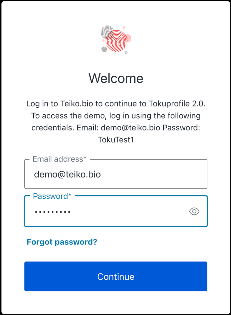
Step 1: Login
Go to app.teiko.bio and sign in with demo credentials: Email: demo@teiko.bio Password: TokuTest1
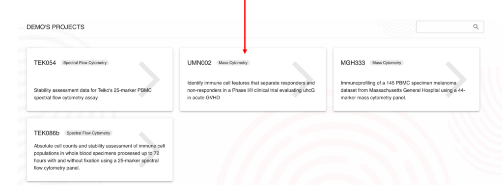
Step 2:
From the list of demo projects, select “UMN002”.
Step 3:
In the navigation menu on the left, select “Data Export”.
2. Select the type of file you would like to download.
3. Select “Append metadata” to include Project-specific metadata for easy downstream data analysis.
4. Optional: Select Normalization baseline. If data should be normalized to a specific time point (e.g. Baseline), normalization can be applied here.
5. Click “Export File”.
6. The file will appear in the downloads tab in the upper right-hand corner.
7. Click the download sign to download the file to your local machine. If Append Metadata is checked, the first 18 columns from this file are project-specific metadata, the following 9 columns are results. The structure of result data is generic and not specific to a project.
High-parameter cytometry has transformed our ability to analyze cell populations by increasing resolution of many subsets, yet the traditional reliance on fresh specimens remains largely unchallenged. The range in stability profiles of different cell subsets, particularly rare populations, necessitate a systematic evaluation of cellular stability. Time between collection and processing affects sample quality, with noticeable differences observed between samples analyzed immediately after collection compared to samples analyzed 72 hours after collection. To accurately determine the freshness of a sample, we propose the term “Fresh-hour”, designating specimens based on their post-collection processing interval, such as “Fresh-0” or “Fresh-72”.
To quantify how processing delays affect sample quality, we analyzed blood from three healthy donors. Each sample was split into four aliquots: one processed immediately after collection (Fresh-0), and the others processed 24, 48, and 72 hours after blood draw (Fresh-24, Fresh-48, and Fresh-72, respectively). All aliquots for each Fresh-X timepoint were analyzed concurrently on a Cytek Aurora spectral flow cytometer. We compared the change in population frequencies at each Fresh-hour time point relative to the baseline, using a 25% change in frequency as the threshold for acceptable variance.
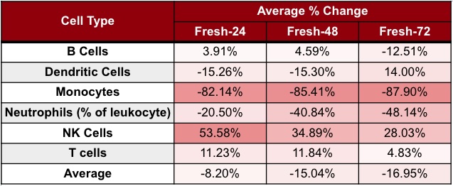
Our analysis showed a linear reduction in the number of live cells from Fresh-0 to Fresh-72, with a 48% reduction in the total cell number by Fresh-72. Cell loss varied by type, with neutrophils and monocytes most affected. When comparing cell population frequencies between Fresh-0 and Fresh-72 for each cell type, we found that the percent of neutrophils decreased by ~48%, and monocytes by ~88% (Table 1).
To assess platform consistency, we evaluated populations from Fresh-3 to Fresh-51 on a Helios mass cytometer. By Fresh-51, all monocyte populations exceeded the 25% threshold. While most lymphocytes remained stable, rare subsets—including double-negative/positive T cells, CD4+ TEMRA, and specific NK and DC populations—showed significant changes. These findings align with the Cytek 25-color immunoprofiling validation report, which found similar changes in rare populations by Fresh-72. Our study demonstrates that Fresh-72 samples differ significantly from Fresh-0 samples, challenging the assumption that all “fresh” specimens are equivalent in high-parameter cytometry.
Table 1. Cell population degradation across processing time points on Cytek Aurora spectral flow cytomer. Values show the average percent change of each cell type at Fresh-24, Fresh-48, and Fresh-72. Fresh-X indicates samples processed X hours after collection.
Short version: no. We are gluttons for gating punishment here at Teiko. We have dozens of quality control checks to make sure that your gating reflects biological reality. Let’s take a tour.
Custom panels: We work out a gating strategy together with you to ensure that all populations of interest are analyzed. Once finalized, we present the gating strategy on a control sample for you to review and approve. If you have changes to make, we can easily incorporate them at this stage.
Standard panels: We review our standard gating scheme with you and you have the ability to make adjustments. This review process ensures that you get correctly gated data.
Post-processing: After samples are processed, we apply your approved gating strategy. We carefully review and adjust (also known as “tailor”) each plot within a sample. This means that we individually adjust thousands of plots per project. After thousands of samples processed, our scientists know when to apply cutoffs. For example, if two patients have different levels of a certain marker, we would need to adjust a gate cutoff. However, if we’re looking at a time-series of an individual, we might need to apply the same cutoff to multiple specimens of that patient to detect changes over time.
This is a crucial step. If we didn’t do this kind of thorough inspection, you would end up with cookie cutter gating, junk data, and ultimately incorrect population measurements.
Independent review: We don’t stop there. Since we like pain, we have another scientist independently review every single plot to make sure nothing gates are placed correctly and nothing gets missed.
See for yourself: After gating, but before we put the data on your dashboard, we present you with compact, letter-size overviews showing the complete gating tree for every sample. This way you can quickly and easily review all gates of an entire sample.
At this point, you have three calendar days to review the gating placement, and request adjustments of gates. This gives you complete visibility into gating and ensures there are no surprises.
Our method gives you total visibility into how your samples are being analyzed at every step of the way. No more rigid reports where you have to spend weeks repairing gating from scratch.
Questions about our gating? Check out free demo datasets at app.teiko.bio.
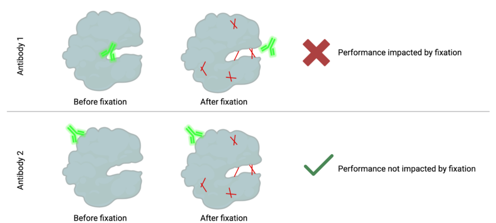
How fixation can mask epitopes: When cells are fixed, the proteins get stuck together in different ways, making it harder for antibodies to reach and bind to the spots (epitopes) they normally would.
In both mass and flow cytometry, the goal is to measure specific immune populations. To measure these populations, we need to detect specific targets, often proteins, within individual cells. This detection relies on labeled antibodies binding to these targets, making them visible to the instrument. Antibodies bind to specific regions on a protein, known as epitopes. However, when samples are chemically fixed to stabilize them for storage, the fixation creates bonds (or methylene bridges) between nearby amino acids in a protein, a process known as cross-linking. These bonds, illustrated in red below, stabilize the protein but can block access to certain epitopes. As a result, some antibodies can no longer recognize their target because their binding region is now “masked.”
Fortunately, proteins have multiple epitopes, and other antibodies may bind to regions unaffected by fixation. These antibodies remain capable of detecting the protein in both fixed and unfixed states. Alternatively, fixation methods without formaldehyde such as methanol-based fixation can be utilized.
When working with fixed samples, it is essential to rigorously test each antibody in your panel to ensure its performance is not compromised by fixation. Proper testing helps ensure accurate and reliable detection of your targets in cytometry assays.
You might have heard of an “immune reset” for Chimeric Antigen Receptor (CAR) therapies in autoimmune diseases. But what does it mean, exactly?
Here’s the 2024 definition from Georg Schett et al’s paper “”Advancements and challenges in CAR T cell therapy in autoimmune diseases”:
“…deep depletion of B cells, including autoreactive B cell clones, could restore normal immune function, referred to as an immune reset.”
Autoimmune diseases, such as systemic lupus erythematosus (SLE), represent some of the hardest conditions to treat. These diseases need lifelong medication with limited success in achieving full remission. But CAR-T is changing that.
In 2022, Schett et al posted this incredible result: “Remission of SLE according to [disease remission] criteria was achieved in all five patients after 3 months and the median (range) Systemic Lupus Erythematosus Disease Activity Index score after 3 months was 0…Drug-free remission was maintained during longer follow-up (median (range) of 8 (12) months after CAR T cell administration).”
From lifelong drugs, to a “one and done” cure.
The concept of an immune reset: “one and done” cure
To make a CAR T-cell therapy, you engineer T cells to target and destroy B cells expressing a target. In the 2022 paper, that was the CD19 antigen. The CD19 antigen turns out to be a key player in many autoimmune diseases. By deeply depleting “autoreactive” B cells, this therapy not only halts disease progression but resets the immune system. (An autoreactive B cell is a type of immune cell that mistakenly recognizes the body’s own tissues as foreign and initiates an immune response against them.)
This approach could yield a one-time cure.
How is an immune reset measured?
It’s an emerging area, so we’re seeing two ways:
Using Cytometry: “Bad” B cells go away, “good” B cells appear
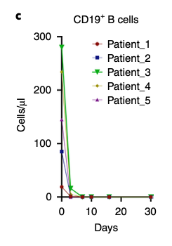
Bad B cell eliminated: Within two days of CAR T-cell infusion, the bad B cells, i.e. CD19+B cells disappeared. Here’s Figure 2c from the 2022 paper:
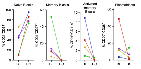
Good B cells appeared: B cells reappeared after an average of 110 ± 32 days but with a big change. These new B cells were predominantly naive (CD21+CD27−) with no memory or autoreactive profiles. (Remember, autoreactive is bad since those kinds of cells attack your own body.) This is Figure 4C from the 2022 paper. BL means Baseline, RC means reconstitution.
Using ELISA: Autoantibody Clearance
Reduction in Anti-dsDNA Levels: Autoantibodies, such as anti-double-stranded DNA (dsDNA), became undetectable in all patients by the three-month mark in the study.
Comprehensive Autoantibody Decline: Beyond dsDNA, other pathogenic autoantibodies, including those targeting nucleosomes and single-stranded DNA, showed similar declines, reflecting a broad reset of immune activity.
Wrapping up
CAR-T has the possibility of being a lifetime “one-and-done” cure to autoimmune disease. It seems that achieving an “immune reset” is a critical step. The science is still evolving, so watch this space!
Goal: Quantitatively measure that blood specimens collected in TokuKit for cytometry remain stable over a period of time.
Of course, we can do this the old-fashioned way, and just wait 24 months. And we are. However, there’s another method, using the Arrhenius equation, which allows us to “accelerate the aging” process. As we measure the “old-fashioned” way, we’ll update our stability assessment accordingly.
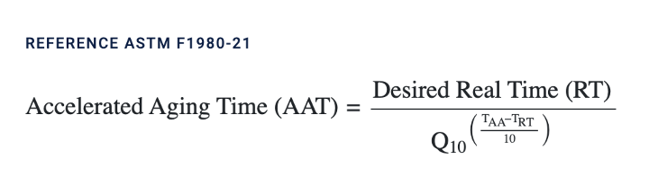
The normal storage temperature for TokuKit is -80°C. For accelerated aging, we used -30°C. We derived the days from the Accelerated Aging calculator, referenced by the American Society for Testing and Materials (ASTM), as follows:
For this, we used TAA = -30C, TRT = -80C, Q10 = 2, and Desired Real Time (RT) = 723 days.
Example 1: in our mass cytometry experiment, we stored the sample at -80°C for one year to naturally age the specimen. We then transferred the sample to -30°C for 12 days to mimic the second year of -80°C storage. This is the “accelerated” part of the experiment.
Example 2: in our spectral flow experiment, we stored the sample at -80°C for 1 week to establish a baseline. We then transferred one aliquot to -30°C for 23 days. This yields the “accelerated” to 2 years, mimicking two years at -80°C.
You just had your IND approved. Now it’s time to look at pharmacodynamic measures. At this point, you want to compare different flow cytometry options. You come back with quotes from two vendors, with these prices per specimen for a gated panel.
Vendor 1: $800 Vendor 2: $1,250
Naive method
Which price is better? Well, this isn’t a trick question: $800 is cheaper than $1,250. $1,250 is 56% more expensive than $800. So yes, Vendor 1 is a better deal. This is the naive way of comparison.
Panel
Cost per specimen
8 marker panel
$800
25 marker panel
$1,250
% Change from 25 to 8
56%
Naive method of comparison
But what if we told you Vendor 1’s panel had 8 markers, and Vendor 2’s panel had 25 markers?
Per marker method
Now, you might compare on a per marker basis.
This is a better way to compare. In this case, you would get $100 per marker for Vendor 1, and $50 per marker for Vendor 2. And in this case, the 25 marker panel is 50% lower than the 8 marker panel.
Panel
Cost per specimen
Number of markers
Price per marker
8 marker panel
$800
8
$100
25 marker panel
$1,250
25
$50
% Change from 25 to 8
56%
-50%
Per marker method of comparison
But, you’re a drug developer and you care about detail in the immune state. You know the immune state means that the more markers you have on your panel, the greater “depth” you can capture in your immune lineage or “tree.”
Price per subset method
That brings us to price per subset.
The 8-marker panel yields 52 subsets while the 25-marker panel produces 298 subsets. This difference dramatically changes the cost-benefit tradeoff. All you need to do is divide the headline price by the number of subsets.
Calculating price-per-subset
Panel 1: $800 / 52 subsets = $15.38 per subset Panel 2: $1,250 / 298 subsets = $4.19 per subset
Let’s see that table again. Now, we can see that using price per subset, the 25 marker panel posts a 73% improvement, compared to an 8 marker panel.
Panel
Cost per specimen
Number of markers
Price per marker
Number of subsets
Price per subset
8 marker panel
$800
8
$100
52
$15.38
25 marker panel
$1,250
25
$50
298
$4.19
% Change from 25 to 8
56%
-50%
-73%
Per subset method of comparison
A simple change in the denominator yields striking differences in the affordability for each panel. Of course, price isn’t the only attribute that matters, but it’s an essential variable that drug developers care about when picking a flow cytometry provider.
How can you use this measure?
If you get different flow cytometry quotes, you might want to use this calculation to get an apples-to-apples comparison.
Are there any limitations to the measure?
This measure just focuses on similar outputs like FCS and gated files. That is, it assumes both methods generate similar outputs. But realistically, drug developers don’t just stop at an FCS file. They need to invest the time or money to turn the FCS file into statistically significant differences. So, this measure doesn’t account for the bioinformatics time or money to turn these FCS files into a true analysis.
Moreover, this measure doesn’t capture sample failure rates, which can impact the actual cost per usable subset. For example, if 10% of samples fail before they even hit a machine with one panel, that would increase your cost per subset downstream.
In sum
The price-per-subset metric is a more realistic way to compare cytometry services. Cytometry’s value is to read more and more detail of the immune “tree”, and by using this measure, you can make better apples-to-apples comparisons between cytometry panels.
What are the advantages of barcoding in mass cytometry? In short, time and money for drug developers.
Here’s an example with 120 specimens. Let’s compare what happens without barcoding and with barcoding.
Parameter
Without barcoding
With barcoding
Processing method
Individual processing per specimen
Samples barcoded and pooled
Number of runs
120 runs (1 per specimen)
6 runs (20 specimens per run)
Data Quality
Variable
Consistent and reliable; reduced cell loss
Figure 1: Comparison of cytometry with and without barcoding
How does barcoding work? Read on to find out.
Example of barcoding in mass cytometry on 120 specimen project
To illustrate how barcoding works in mass cytometry, let’s consider a simple example on the 120 specimen project using metal isotopes for tagging samples.
Goal: Barcode 20 different samples for simultaneous analysis. Remember, we had a 120 specimen project, with 20 specimens in each of the six runs.
First, the barcode criteria must be established:
Purity: each isotope must be >90% pure Titration: each isotope is titrated to the concentration that gives the best signal-to-noise ratio. This is similar to what we do with antibodies. We also ensure each isotope produces similar “brightness.” Combination: after each isotope is titrated, combine three isotopes together into one barcode and test again the optimal concentration to be stained with cells
Second, we pick the barcoding isotopes: We’ll use six palladium isotopes not used in the 40+ marker antibody panel. To construct the actual barcode, we’ll pick three from those six, to avoid signal overlap between the channels. ¹⁰²Pd ¹⁰⁴Pd ¹⁰⁵Pd 106Pd 108Pd 110Pd
Now, the fun part starts.
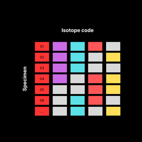
Third, we build a barcoding scheme:
By using different combinations of these three isotopes, we can create unique barcodes for each sample. Here’s an example:
Mass in Angstroms
Specimen ID
102
104
105
106
108
110
01
1
1
1
0
0
0
02
1
1
0
1
0
0
03
1
1
0
0
1
0
04
1
1
0
0
0
1
05
1
0
1
1
0
0
06
1
0
1
0
1
0
07
1
0
1
0
0
1
08
1
0
0
1
1
0
09
1
0
0
1
0
1
10
1
0
0
0
1
1
11
0
1
1
1
0
0
12
0
1
1
0
1
0
13
0
1
1
0
0
1
14
0
1
0
1
1
0
15
0
1
0
1
0
1
16
0
1
0
0
1
1
17
0
0
1
1
1
0
18
0
0
1
1
0
1
19
0
0
1
0
1
1
20
0
0
0
1
1
1
Figure 2: Barcodes by Sample
Fourth, onto the actual processing steps in the lab:
Barcode individual samples: Each of the 20 samples is incubated separately with a specific combination of the barcoding isotopes from the table above. The isotopes bind to proteins uniformly across all cell types in the sample.
Pool samples: After barcoding, all 20 samples are combined into a single tube. The pooled sample is then stained with a panel of metal-tagged antibodies targeting specific cellular markers (using different isotopes not overlapping with the barcodes).
Acquire the data: The pooled, stained sample is run through the mass cytometer. The cytometer detects the metal isotopes from both the barcodes and the antibody-bound markers.
Deconvolve the data: Specialized software analyzes the data, identifying cells based on the presence of barcoding isotopes. Cells are assigned back to their original samples according to the unique combination of isotopes detected. For example, a cell positive for 102Pd, 104Pd for 110Pd is assigned to Specimen 04.
And then, analyze! Once deconvoluted, each sample’s data can be analyzed individually for immunophenotyping. This includes assessing the expression of various markers to characterize cell populations.
So what just happened?
A drug developer who sends 120 specimens, can get them done in 6 runs, not 120. That means lower batch variation, and better quality data for your patients.
Bonus: what if we need more barcodes?
You might have noticed that we used 6 isotopes to generate barcodes, which yields 20 combinations (6 Choose 3). As the number of specimens per run increases, you can add more isotopes to generate higher combinations (i.e. 10 isotopes can generate 120 combinations).
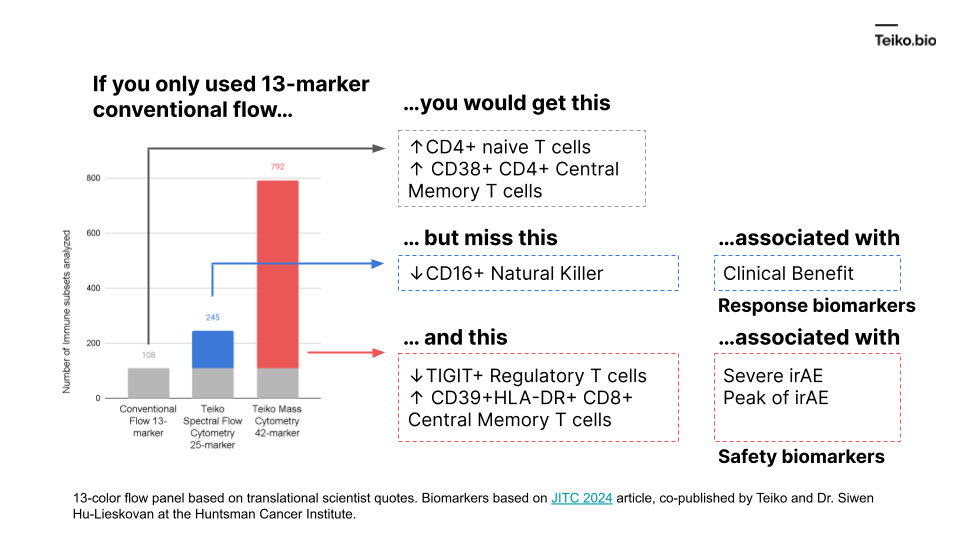
“I have a 13 marker panel that analyzes T-cells. And my drug just hit the T-cells, why bother looking at any other immune cell types, like B cells, or NK cells? Even if those other cells are affected, I don’t know how to interpret those results.”
The reason is: those extra subsets might predict the difference between success and failure for a drug.
More to the point, if we took a conventional flow panel, you get up to ~108 subsets with a 13-marker panel, almost exclusively T cells. Using mass cytometry, with a 42-marker panel, you get to 792. With spectral flow, it’s around 245. This diagram shows what is missed by the lower-parameter methods. And these are cell subsets we ourselves have found in our own work and collaborations, associated with either clinical benefit, severe immune-related adverse events or peak toxicity.
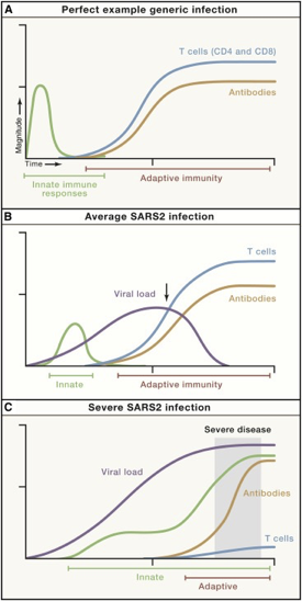
We know there is a “characteristic” time-series curve associated with clearing infections, like COVID. It would be difficult for a drug developer to analyze a “productive” immune response if whole curves were missing. For example, imagine tracking one curve, like the antibodies. If you tracked just antibodies, you could be misled into thinking someone had an average COVID infection or generic infection.
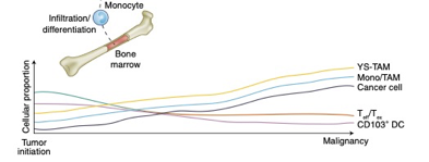
There is good reason to believe this sort of curve is true in cancer immunology. To that point, this is a nice time-series diagram from Nature Medicine of different cell types in the tumor microenvironment. The authors summarized it well: “understanding what cell types can be modulated and when may enable the next biggest improvements in immunotherapy.”
These distinct subtypes are not of academic interest: these drive real-world responses.